This post is the final part of a three-part miniseries that looks at how we improved join performance in the CrateDB 3.0 release.
In part one of this miniseries, I went over the reasons we chose to implement the hash join algorithm as an alternative to the nested loop algorithm. With that initial set of changes in place, we were able to make joins up to two thousand times faster.
In part two, I explained how we addressed the memory limitations of the basic hash join algorithm with a switch to block-based processing. That is, dividing a large dataset up into smaller blocks that can be worked on separately. On top of that, we managed to improve our performance by an average of 50% by switching the joined tables so that the smaller table is on the right-hand side.
This brings us to the final set of changes.
With the work so far, the CrateDB node that handles the client request is responsible for planning and executing the entire join.
However, because we now have blocks that can be worked on separately, we can, in theory, distribute those blocks across the CrateDB cluster and execute the join in parallel using multiple nodes for increased performance and load distribution.
To put it another way, what we needed to do was modify our existing implementation so that it (as evenly as possible) distributes the work required for the block hash join.
In this post, I will show you how we modified our existing work to create a distributed block hash join algorithm. I will then present the results of our final benchmarks.
Please note: join algorithms and their performance characteristics are common knowledge for RDBMS developers. This miniseries is written for people who want a behind the scenes look as we implement these algorithms and adapt them for CrateDB and our distributed SQL query execution engine.
Approaches
We identified two candidate approaches for this work:
- The locality approach
- The modulo distribution approach
In this section, I will explain each approach, and then present the results of our prototyping benchmarks.
The Locality Approach
In an ideal situation, a CrateDB table is split up into primary shards that are distributed evenly across each node in the cluster.
If we have a table with eight shards, and a cluster with three nodes, we might expect a distribution that looks like this:
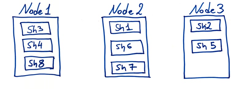
Ideally, tables also have replication configured, which means that each primary shard should have one or more replicas, which can also be used for read operations. However, I have omitted this from the diagram above to keep the explanation simple.
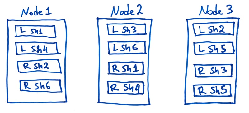
If you are joining two tables, you have two such tables, and two sets of shards that are distributed across the cluster.
For distributed query execution, ideally, each node in the cluster should perform a portion of the work required for the join.
One of the consequences of the block hash join algorithm (as detailed in part two) is that the left (outer) table is split into blocks and the right (inner) table must be read once for every block. To minimize the total number of rows read, we swap the tables if necessary to ensure that the right-hand table is the smallest of the two.
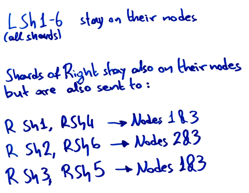
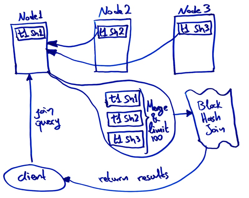
So, for the locality approach, each node must:
- Identify the left-hand table shards that are kept locally and then split those shards into blocks.
- Broadcast the right-hand table shards that are kept locally to all other nodes.
- Use the complete set of rows for the right-hand table, taken from the shards residing locally on the node and the ones received from other nodes.
- Produce a partial result set by running the hash join algorithm on the local left-hand blocks using the local copy of the right-hand table.
Partial result sets are then transmitted to the handling node for merging and further processing (e.g., applying operations like ORDER BY, LIMIT, OFFSET, and so on) before being returned to the client.
Here's what that looks like:
The Modulo Distribution Approach
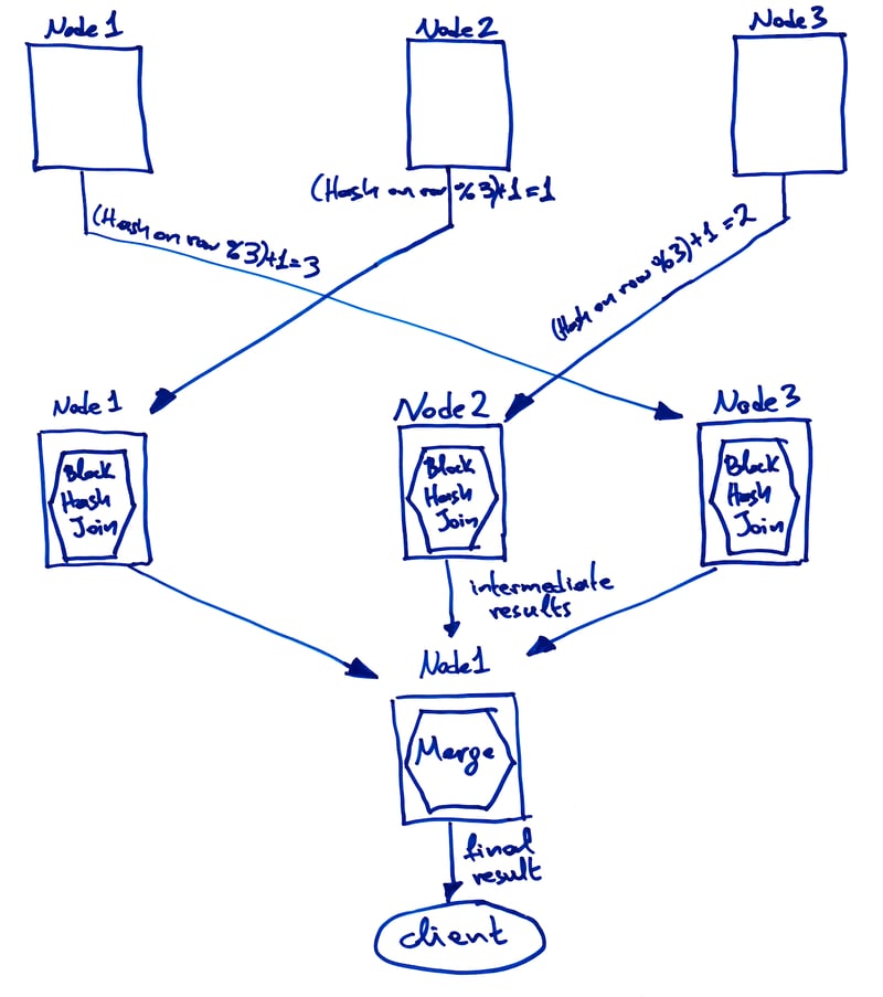
The grace hash join algorithm inspired our modulo distribution approach.
The basic idea is that every node produces a hash for every local row in every local shard for both tables participating in the join. This hashing is done in a way that ensures that matching rows will have a matching hash. We then modulo the hashes to partition the matching rows across the cluster.
This method ensures that every right-hand row is located on the node that also holds every potentially matching left-hand row. As a result, every node can split its assigned subset of left-hand rows into blocks and execute a hash join using only its assigned subset of right-hand rows.
Take the following query:
SELECT *
  FROM t1
  JOIN t2
    ON t1.a = t2.a + t2.b
   AND t1.b < t2.c
As discussed in part one, we're interested in equality operators. So in this example, this is what we care about:
t1.a = t2.a + t2.b
Using this equality operator, we would calculate the hash for rows in t1 using the value of a, and a hash for rows in t2 using the value of a + b.
Because we're using an equality operator, matching rows from t1 and t2 will have identical hashes.
From here, we can assign each row to a node using the modulo operator, like so:
node = hash_value % total_nodes
Statistically speaking, the modulo operator will assign approximately the same number of rows to each node in the cluster.
So, to summarize, for the modulo distribution approach, each node must:
- Calculate the appropriate hash for every row for every local shard for both tables participating in the join.
- Assign every row to a node by taking a modulo of the hash.
- Transmit rows to their assigned nodes, as necessary.
- Assemble the subset of assigned left-hand and right-hand rows from the rows held locally and the rows received from other nodes in the cluster.
- Produce a partial result set by running the block hash join algorithm on the assigned subsets of left-hand and right-hand rows.
As before, partial result sets are then transmitted to the handling node for merging and further processing before being returned to the client.
Here's what the whole thing looks like:
Making a Decision
To test the two approaches we benchmarked two prototyped implementations on a five node CrateDB cluster.
For our benchmarks, the left (outer) table, t1, held 20 million rows, and the right (inner) table, t2, held five million rows.
We ran the following query:
    SELECT *
      FROM t1
INNER JOIN t2
        ON t1 = t2
Using three algorithms:
- The original single-node block hash join algorithm
- The locality prototype
- The modulo distribution prototype
With four different table configurations:
- Three primary shards, no replicas
- Five primary shards, no replicas
- Five primary shards, one replica each
- 10 primary shards, one replica each
And three different LIMIT values:
- 1,000
- 10,000
- 100,000
Here's what we saw:
| Execution Time (seconds) | ||||
|---|---|---|---|---|
| Configuration | Limit | Single Node | Locality | Modulo |
| Three primaries, no replicas | 1,000 | 1.465 | 5.658 | 1.210 |
| 10,000 | 1.579 | 5.890 | 1.569 | |
| 100,000 | 4.017 | 8.916 | 3.722 | |
| Five primaries, no replicas | 1,000 | 1.610 | 3.985 | 1.332 |
| 10,000 | 2.048 | 4.759 | 1.642 | |
| 100,000 | 4.868 | 8.202 | 3.490 | |
| Five primaries, one replica each | 1,000 | 1.488 | 5.999 | 1.409 |
| 10,000 | 1.809 | 6.487 | 1.873 | |
| 100,000 | 5.016 | 10.394 | 3.678 | |
| 10 primaries, one replica each | 1,000 | 1.413 | 3.286 | 1.324 |
| 10,000 | 1.792 | 4.351 | 1.655 | |
| 100,000 | 4.493 | 6.580 | 3.220 | |
From this, we can observe that:
- The locality approach would not improve performance over the original single-node block hash join algorithm. In fact, it worsens performance.
- The modulo distribution approach improves performance for all tested configurations.
The results showed that the locality approach wouldn’t improve performance over the single node execution but on the contrary, would make it slower. On the other hand, the modulo distribution would improve performance for all tested configurations over the single node execution.
This was in line with what we were expecting, for two reasons:
- The locality approach can easily generate a lot of internal traffic because every node must receive all right-hand rows that exist on other nodes.
- The modulo distribution approach reduces the total number of row reads because each node only has to compare its assigned subsets of left-hand and right-hand rows. Contrast this with the locality approach which still requires the hash join algorithm to compare against the whole right-hand table for every block.
With these results in hand, we decided to go with the modulo distribution approach.
Thankfully for us, CrateDB's existing distributed query infrastructure made light work of this implementation, so details of the code changes we made can be skipped for this post.
A Precautionary Limitation
We identified one potential issue during implementation.
If you are joining a subselect, and that subselect has a LIMIT or an OFFSET clause, the distributed algorithm may perform worse than the single-node version.
To understand why let's take an example query:
SELECT *
  FROM (
    SELECT a
      FROM t1
     LIMIT 100) AS tt1,
  JOIN t2
    ON tt1.a = t2.b
When a single node is executing this query, it only needs to collect 100 rows for t1 before being able to complete subselect and proceed with the join.
Here's what that might look like:
However, we can't do this with the distributed block hash join algorithm, because each node is only processing a subset of the data.
For us to complete the subselect as before, one of the nodes would have to complete the subselect by receiving all data for t1 and apply the limit of 100 before distributing the rows across the cluster to proceed with the execution of the distributed block hash join algorithm.
We decided this was out of the scope for this work, and so instead we applied a limitation so that the single-node version of the block hash join algorithm is used instead of the distributed version for any query joining a subselect with a LIMIT or an OFFSET.
Benchmarks
With the implementation of the distributed block hash join algorithm complete, we performed a final set of benchmarks to compare it with the single-node version.
Like before, we used a five node CrateDB cluster.
This time, we created two tables, t1 and t2, configured with five primary shards each and no replica shards.
For the first test iteration, both tables started out with 10 thousand rows, and this was increased for every subsequent iteration.
For each iteration, we tested two queries using three algorithms:
- The original nested loop algorithm
- The single-node block hash join algorithm
- The distributed block hash join algorithm
The first query matches all rows:
     SELECT COUNT(*)
      FROM t1
INNER JOIN t2
        ON t1.a = t2.a
The second query was designed to match one-fifth of all rows using a second column that was populated accordingly:
     SELECT COUNT(*)
      FROM t1
INNER JOIN t2
        ON t1.a = t2.a
       AND t1.b = t2.b
Every combination of query, table size, and algorithm was run multiple times and the average execution time was taken.
The results were as follows:
| Execution Time (seconds) | Modulo Improvement | |||||
|---|---|---|---|---|---|---|
| Rows | Match | Nested Loop | Single Node | Modulo | vs. Single Node | vs. Nested Loop |
| 10,000 | All | 1.7411 | 0.01587 | 0.01447 | 1.096x | 120x |
| ⅕ | 2.5379 | 0.01422 | 0.01160 | 1.225x | 218x | |
| 20,000 | All | 6.3593 | 0.02434 | 0.02138 | 1.138x | 297x |
| ⅕ | 9.7377 | 0.01969 | 0.01597 | 1.232x | 609x | |
| 50,000 | All | 39.5819 | 0.04643 | 0.04155 | 1.117x | 952x |
| ⅕ | 60.9723 | 0.04194 | 0.03068 | 1.366x | 1987x | |
| 100,000 | All | 158.6330 | 0.08921 | 0.06773 | 1.317x | 2342x |
| ⅕ | 242.1353 | 0.06922 | 0.05169 | 1.338x | 4683x | |
| 200,000 | All | 628.5157 | 0.13737 | 0.11172 | 1.229x | 5625x |
| ⅕ | 1025.8460 | 0.12579 | 0.08842 | 1.422x | 11601x | |
| 500,000 | All | 3986.6020 | 0.35814 | 0.17324 | 2.067x | 23011x |
| ⅕ | N/A | 0.31457 | 0.24539 | 1.281x | N/A | |
| 1,000,000 | All | N/A | 0.79487 | 0.46546 | 1.707x | N/A |
| ⅕ | N/A | 0.67291 | 0.29302 | 2.296x | N/A | |
Note: tests marked N/A ran for too long and were terminated.
From this, we can observe that:
- The original nested loop algorithm performs reasonably for tables with up to 500 thousand rows.
- For tables with more than 50 thousand rows, the distributed block hash join algorithm is significantly faster than the single-node block hash join algorithm.
- For tables with less than 50 thousand rows, the performance benefits of the distributed block hash join algorithm do not outweigh much the associated performance costs, i.e., distributing rows internally, and so on.
- The distributed block hash join algorithm makes join operations up to 23 thousand times faster than they are with the nested loop algorithm.
Huge success!
Further Benchmarking
We didn't want to stop here. So, we devised some additional benchmarks.
Specifically, we used the same basic setup for the tests, but this time we ran the queries individually and then 10 times simultaneously to simulate multiple concurrent users. We also increased the size of the test tables in steps.
The results were as follows:
| Rows | Match | Concurrency | Execution Time (seconds) |
| 2,000,000 | All | 1 | 1.65599 |
| 10 | 3.96610 | ||
| ⅕ | 1 | 1.41749 | |
| 10 | 3.90570 | ||
| 5,000,000 | All | 1 | 3.41488 |
| 10 | 7.89427 | ||
| ⅕ | 1 | 3.32135 | |
| 10 | 6.92028 | ||
| 10,000,000 | All | 1 | 8.89686 |
| 10 | 19.27493 | ||
| ⅕ | 1 | 8.39930 | |
| 10 | 18.45803 | ||
| 20,000,000 | All | 1 | 25.33473 |
| 10 | 50.41725 | ||
| ⅕ | 1 | 23.53943 | |
| 10 | 47.99202 | ||
| 50,000,000 | All | 1 | 129.59995 |
| 10 | 171.60423 | ||
| ⅕ | 1 | 113.96354 | |
| 10 | 160.43524 |
Interpreting these results is more subjective because we're not comparing them with any previous results. We are, however, happy with this performance profile because many of the typical real-world CrateDB deployments have tables with millions of rows.
Wrap Up
In parts one and two of this miniseries, we walked you through our implementation of the hash join algorithm, and how we subsequently improved on that work with the block hash join algorithm.
In this post, I showed you how we took the block hash join algorithm and modified it to run in parallel on multiple nodes.
We shipped this work in CrateDB 3.0, and the result is that inner joins with equality operators are significantly faster in all cases.
23 thousand times faster in some cases.
There are some potential improvements we could make:
- Implementing semi-joins and anti-joins with a hash join algorithm could improve performance enough to make them viable as a general query optimization strategy.
- Revisit and implement the sorted merge join algorithm, which could significantly improve the performance of inner joins with equality operators and an
ORDER BYclause as well as inner joins that do not use equality operators. - A helpful Reddit user suggested that bloom filters would reduce the number of blocks the block hash join algorithm produces.
We don't have anything roadmapped at the moment, but as always, stay tuned. And if you have suggestions for further improvements we could make, or you would like to contribute to CrateDB and make improvements yourself, please get in touch!