In a recent batch of work, we added support for joining on virtual tables, and support for multi-row subselects. That work is available in the latest CrateDB.
In this post, I will introduce you to both concepts, explain the challenges we faced, and show you how we implemented them.
One of those challenges was big enough that it gets a whole section of this post dedicated to it. The summary is that memory can become a bottleneck for some multi-row subselects. Fortunately, we found a neat solution.
Keep reading to learn more.
Joins on Virtual Tables
Joining on virtual tables is a crucial feature for many users, and it is especially useful when doing analytics on your data.
What is a virtual table? It's what we call the result set returned by a subquery.
So, for example, here's a join across two regular tables:
     SELECT *
       FROM table_1
 INNER JOIN table_2
         ON table_1.column_a = table_2.column_a
      WHERE table_1.column_b > 10
In previous versions of CrateDB, these were the only sort of tables you could join across.
But we wanted to add support for queries like this:
    SELECT *
      FROM (SELECT *
              FROM table_1
          ORDER BY column_a
             LIMIT 100)
        AS virtual_table_1,
INNER JOIN (SELECT *
              FROM (SELECT *
                      FROM table_2
                  ORDER BY column_b
                     LIMIT 100)
                AS virtual_table_2
          GROUP BY column_c)
        AS virtual_table_3
     ON virtual_table_1.column_a = virtual_table_3.column_a
What's going on here? Well, instead of joining on regular tables (also known as base tables), we are joining on result sets returned from two subselects (in fact, one of the subselects has a nested subselect, just to give you an idea of what is possible!)
Being able to use subselects as virtual tables for the lifetime of a query is very useful because it means that you can slice and dice your data multiple ways without having to alter your source data, or store duplicate version of it.
But enough of that. How did we make this possible?
Well, we had to do the following things:
- Refactor, refactor, refactor
- Make sure we handle push-downs correctly
- Make changes to the query planner
Refactoring
First some background.
After being successfully parsed, every SELECT statement is processed by the Analyzer class and gets modeled as a QueriedRelation object. Every join within that statement is modeled as a MultiSourceSelect object (a subclass of QueriedRelation ). These MultiSourceSelect objects list a number of sources, one for every table that participates in the join.
Previously, the sources of a MultiSourceSelect were modeled by a RelationSource class, and this class didn't support virtual tables.
So the first thing we had to do was swap out RelationSource objects for the more generic QueriedRelation objects, which can handle virtual tables. To accomplish this, we had to refactor the Analyzer class and the Planner class to accommodate the change.
Push-Downs
When analyzing and planning a join, we try to "push down" operations such as WHERE, ORDER BY and LIMIT to the tables of the join.
This helps to improve performance.
Why?
Because:
- For
WHEREclauses, the sooner we apply this operation, the sooner we can filter out irrelevant records. - For
ORDER BYclauses, if we can push these down to the base-table level we can get our results pre-ordered for us by the storage engine. - For
LIMITclauses, the sooner we limit rows, the less work that subsequent operations have to do.
For example, when the user specifies LIMIT 100, by pushing this down, we make sure that at any time, we never select more than 100 records from the queried tables.
We say "push down", because this information comes from the outer scope of the query and is "pushed" down to the inside scope.
If we didn't push down operators, we could end up selecting much more data than is necessary, slowing the whole query down, often by orders of magnitude.
Take this query, for example:
    SELECT *
      FROM table_1
CROSS JOIN table_2
  ORDER BY table_1.column_a
     LIMIT 100
Since this is a cross join, we can pre-order the rows of table_1. That's because table_1 is on the left-side of the nested loop operation that implements the join.
We can also apply a limit 100 to both tables, since 100 times 100 is more than the final number of rows (100) we are meant to return.
At this point, you might be thinking that it makes sense to push down a limit of 10. As 10 times 10 equals one hundred, and that's the final limit value.
However, this is not safe. Because we don’t know how the data is distributed across the two tables.
For example, consider the case when one table has only nine records and the other table has 1,000. If we push down a limit of 10 to both tables, we will get back nine times 10, i.e. 90 records. This is less than the specified 100 records.
Internally, the above query is rewritten and executed as this:
    SELECT *
      FROM (SELECT *
              FROM table_1
          ORDER BY table_1.column_a
             LIMIT 100)
        AS virtual_table_1
CROSS JOIN (SELECT *
              FROM table_2
             LIMIT 100)
        AS virtual_table_2
But, let's say you're starting with a top-level query that looks like this:
    SELECT *
      FROM (SELECT *
              FROM table_1
          ORDER BY table_1.column_a
             LIMIT 100)
        AS virtual_table_1
CROSS JOIN (SELECT *
              FROM table_2
             LIMIT 100)
        AS virtual_table_2
  ORDER BY column_b
     LIMIT 10
Notice the additional ORDER BY and LIMIT 10 on the outer query? We can't push that down into subselects without changing their semantics. So there *is* a limitation on when those push-down optimizations can be applied.
The introduction of virtual tables adds more complexity to the decision about whether to push down an operator or not. So we had to modify the LogicalPlanner to be able to handle this additional complexity.
Changes to the Query Planner
As previously mentioned, in the past, the sources of a MultiSourceSelect have always been base tables, not virtual tables (i.e. resulting from a subselect). Base tables do not need any additional operations on top before the result set is available.
Virtual tables, however, by nature of being generated by a subselect, can require additional operations. For example, ORDER BY, LIMIT, GROUP BY, as well as aggregate functions like MAX(), SUM(), COUNT(), and so on.
Internally, these operations are modeled by classes such as TopNProjection, AggregationProjection, and MergePhase. And to do this, the query planner had to be changed to check for those operations and plan them in the correct order so that they are executed before the join operation.
Multiple Row Subselects
In older versions of CrateDB we only had support for selecting a single column from a single row in a subquery. For example:
SELECT table_1.*,
       (SELECT MAX(column_b) FROM table_2) AS max_column_b
  FROM table_1
 WHERE column_a > (SELECT MIN(column_b) FROM table_2)
Internally, these subselects are marked with a special placeholder (SelectSymbol) so that the query planner can recognize them and produce a special MultiPhasePlan.
A MultiPhasePlan, as the name suggests, is executed in multiple steps.
Firstly, the subselects are executed. And then the values produced by those subselects are replaced into the SelectSymbol placeholders. Once this is done, the top-level query is executed.
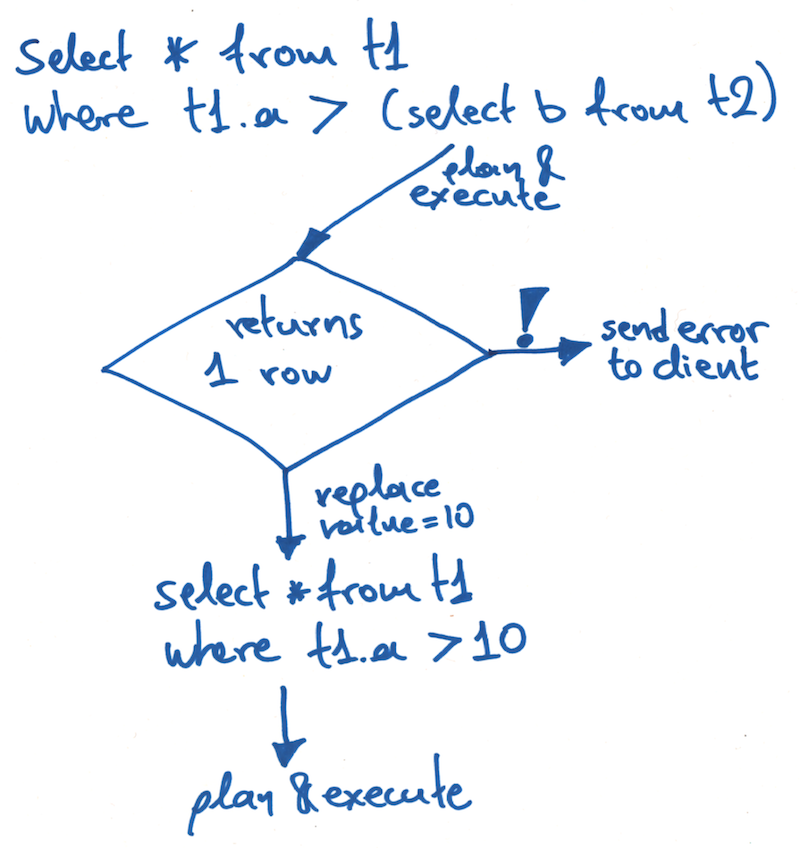
Since we know that these subselects should only produce one row, the planner applies a LIMIT 2 to them automatically. The results are then handled by a special SingleValue collector that will throw an error as soon as more than one row is produced.
Why? Because more than one row means that the query is unsuitable and an error must be raised to the user.
We don't care how many rows are produced, only that it is more than one. And by limiting the query and erroring immediately, the planner can avoid potentially calculating millions of result rows unnecessarily.
Here's a quick sketch of how a single-row subselect works:
However, for this batch of work, we wanted to expand our handling of subselects so that they do support queries that return more than one row. This is useful because it allows queries to use the ANY() function to check whether a value is contained within the result set produced by a subquery.
For example:
SELECT *
  FROM table_1
 WHERE column_a = ANY(SELECT column_b FROM table_2)
To implement this, we had to modify the query analyzer to recognise this new type of subselect that returns multiple rows. The analyzer must then mark the SelectSymbol placeholder object with the correct ResultType class indicating that it returns a multi-row value.
We then had to modify the query planner to check the ResultType class. If it's a single-row value, it is handled like before. If it is a multi-row value, the LIMIT 2 is not applied, and instead a new AllValues collector is used to collect the results.
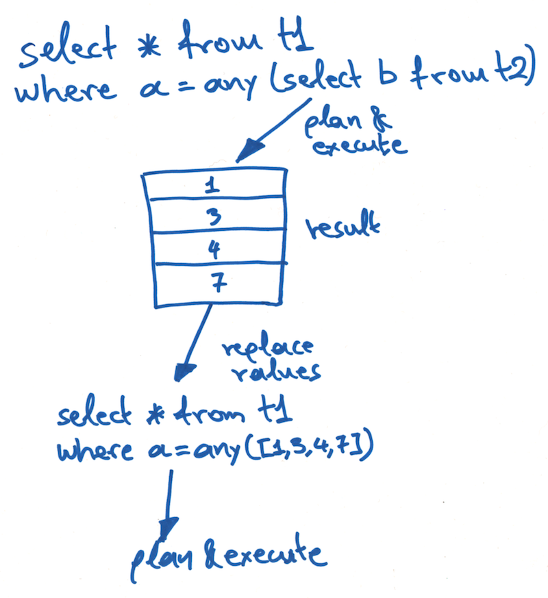
Once all the rows have been collected, they are replaced into the top-level query as a list of literals.
For example, the previous query might end up being rewritten like this:
SELECT *
  FROM table_1
 WHERE column_a = ANY([2, 4, 6, 8])
Here's a quick sketch of how the new multi-row subselect works:
As a bonus, we added IN() support by rewriting these functions using ANY().
So, this query:
SELECT *
  FROM table_1
 WHERE column_a IN (SELECT column_b FROM table_2)
Ends up being rewritten as this:
SELECT *
  FROM table_1
 WHERE column_a = ANY(SELECT column_b FROM table_2)
Semi Joins and Anti Joins
When a multi-row subselect produces a large number of rows (e.g. millions) those rows need to be held in-memory on one node before they can be replaced into the outer query. And this can easily lead to out-of-memory issues.
To deal with this, we decided to rewrite these queries internally using semi joins and anti joins.
The plans created are no longer using the MultiPhasePlan class, which is executed in two steps (first the subquery and then the top-level query). Instead, we use the NestedLoopPlan class (with a flag denoting join type) which is executed in one step, without needing to temporarily store the intermediate result rows produced by the subquery.
This effectively addresses any potential memory issues.
So, a query like this:
SELECT *
  FROM table_1
 WHERE column_a IN (SELECT column_b FROM table_2)
Is rewritten internally, like this:
   SELECT *
     FROM table_1
SEMI JOIN table_2
       ON table_1.column_a = table_2.column_b
And this:
SELECT *
  FROM table_1
 WHERE column_a NOT IN (SELECT column_b FROM table2)
Is rewritten like this:
   SELECT *
     FROM table_1
ANTI JOIN table_2
       ON table_1.column_a = table_2.column_b
Note: SEMI JOIN and ANTI JOIN syntax are not available for user queries. These are internal join types only and are always the result of an internal query rewrite.
To implement this feature we introduced added an optimizing rewriter.
The New Optimizing Rewriter
We introduced a new class, OptimizingRewriter, which is responsible for preprocessing the AnalyzedStatement object before the actual planning takes place. The rewriter detects the aforementioned subselects and decides if a rewrite to a semi or anti join is possible.
If the subselects are being used with IN() or ANY() as part of an OR condition, the query cannot be rewritten to a semi or an anti join.
Take this query, for example:
SELECT *
  FROM table_1
 WHERE column_a IN (SELECT column_b FROM table_2)
    OR column_c IN (SELECT column_d FROM table_3)
If we wanted to rewrite this query as a semi join, table_1 would have to be "simultaneously" joined with table_2 and table_3 so that each row of table_1 could be checked against all rows of table_2 and all rows of table_3 to decide if it meets the select criteria.
This hypothetical 3-way join is not a valid relational algebra operator and would have been extremely inefficient to implement. So, these types of queries are always executed in multiple steps using the MultiPhasePlan as described before.
On the other hand, if OR is replaced with AND, like this:
SELECT *
  FROM table_1
 WHERE column_a IN (SELECT column_b FROM table_2)
   AND column_c IN (SELECT column_d FROM table_3)
The query can be rewritten as two semi joins:
SELECT *
     FROM table_1
SEMI JOIN table_2
       ON table_1.column_a = table_2.column_b
SEMI JOIN table_3
       ON table_1.column_c = table_3.column_d
When a valid rewrite opportunity is detected, the OptimizingRewriter creates a MultiSourceSelect (used to model all types of joins) and sets table_1 and table_2 as the source tables. It also constructs a JoinPair with JoinType set to JoinType.SEMI and a JoinCondition or table_1.id = table_2.id.
This JoinPair is also saved in the MutliSourceSelect instance which is now ready to be passed along to the LogicalPlanner. The LogicalPlanner in turn reads this information from the JoinPair and properly create a plan for the semi or anti join operation which is now ready for execution.
Execution Details
Digging into the core execution layer, each type of join operation (cross, inner, left, right, and full) is implemented by a JoinBatchIterator. Each type of JoinBatchIterator operates on two source BatchIterators, the left and the right. These provide rows from the left and the right tables respectively.
Semi and anti join operations were implemented using the NestedLoop algorithm. So, two new NestedLoopBatchIterator classes (a subclass of JoinBatchIterator) were introduced: SemiJoinBatchIterator and AntiJoinBatchIterator.
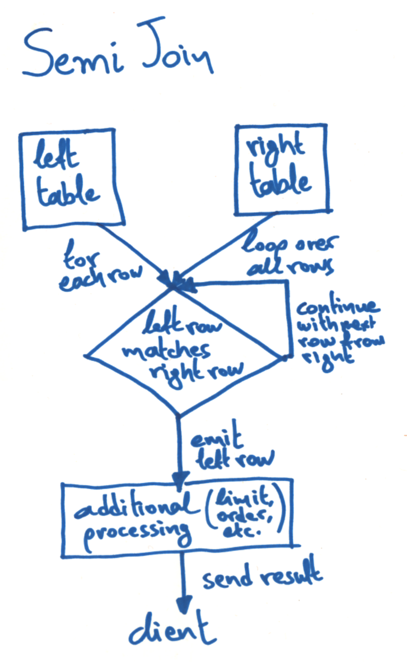
The SemiJoinBatchIterator implements the semi join by reading the rows of the left table one-by-one, and for each one it loops over the rows of the right table. If a match is found, we exit the secondary loop and emit the matching left table row.
Here's a quick sketch the corresponding flow diagram:
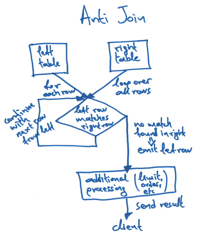
The AntiJoinBatchIterator implements the anti join by reading the rows of the left table one-by-one, and for each one it loops over the rows of the right table. If a match is found, we exit the secondary loop and move on to the next row of the left table. If no match at all is found in the right table, the corresponding row from the left table is emitted.
Here's a quick sketch of the flow diagram for an anti join:
Disabled By Default
If you have a memory bottleneck, these rewritten queries are likely to significantly improve performance. But if you do not have a bottleneck, the performance of these rewritten queries is going to be worse than using the original multi-phase execution.
For that reason, rewriting queries to semi joins and anti joins is still an experimental feature and is only meant to be used when the situation calls for it.
If you want to enable it in the latest versions of CrateDB, you must set the session variable semi_joins to true. This will hint the OptimizingRewriter to check for valid semi join and anti join rewrite opportunities.
Wrap Up
To add support for joins on virtual tables we had to refactor our code, make sure we were handling push-down operations correctly, and then make modifications to the query planner.
We also made changes to the query planner to add support for multi-value subselects which you can now use as arguments to ANY() and IN().
And finally, we added a new optimizing query rewriter that optimizes the execution of some memory bottlenecked subquery operations.
All of this is available in the latest version of CrateDB, so you can download immediately and start playing.